Mixture-of-Quantization: A novel quantization approach for reducing model size with minimal accuracy impact

A unified suite for quantization-aware training and inference

Running large-scale models on multi-GPU might help reduce latency but increases the deployment cost significantly, especially as the model size grows bigger. To mitigate this issue, we resort to model compression techniques and introduce a new methodology that quantizes Transformer networks with a minimal impact on accuracy. Our technique achieves similar or better performance thanFP16 models through customized inference kernels on lower or equal number of GPUs.

Our scheme is flexible in the sense that it provides users the ability to experiment with any quantization configuration, such as the target number of bits used for quantization precision, and the scheduling by which the model gets quantized during training. Furthermore, we combine both the FP16 and quantized precision as a mixed-precision mechanism to smooth the transition from a high to low precision. Finally, we use the second-order gradient (eigenvalue) of the parameters to adjust the quantization schedule during training.

Quantization methodology

There are two main approaches of applying quantization: offline quantization on the trained model and quantization-aware training (QAT) that reduces the data-precision during training. Unlike the former scheme, QAT gets the model trained by taking the impact of precision loss into account during the training optimization. This will result in significant improvement of the quantized model accuracy. MoQ is designed on top QAT approach, with the difference that we use a mixture of precisions to train the model toward target quantization, as well as defining a scheduling for reducing the precision.

All existing QAT approaches quantize the model with a certain precision (number of bits) from the beginning of training until completion. However, even by using a relatively high quantization precision (8-bit), there will be some drop in model accuracy, which might not be acceptable for some downstream tasks. For instance, the Q8BERT work tries QAT for the BERT network, which results in good accuracy for some tasks while others (like SQuAD) lose 0.8% in the F1 score. Other techniques, such as Q-BERT, use grouped quantization with a large grouping size (128) when quantizing a parameter matrix to gain higher accuracy, but they are still inferior to the baseline.

Here, we present MoQ as a flexible solution for linear quantization that allows users to define a schedule as the model trains. Similar to iterative pruning to inject sparsity, we start quantization from a higher precision (16-bit quantization or FP16) and gradually reduce the quantization bits or the mixed-precision ratio for the FP16 part until reaching a target precision (8-bit). To control the precision transition, we define a hyperparameter, called quantization period, that indicates when the precision reduction should happen. We observe that by using such a schedule, we get the closest accuracy to the baseline. Note that in order to reach a certain precision, we need to define the starting bits and period in a way that within the number of samples to train, the model eventually gets quantized using the target number of bits. Please refer to the quantization tutorial for more information.

In order to dynamically adjust quantization precision, we employ eigenvalue as a metric that shows the sensitivity of training to the precision change. Eigenvalue has been previously used (Q-BERT) for quantization to choose the precision bits on different parts of the network. To combine this with MoQ, we cluster the eigenvalues into several regions based on their absolute values and tune the quantization period for each region accordingly, the higher the magnitude of eigenvalue, the larger the factor and the slower the precision decreases.

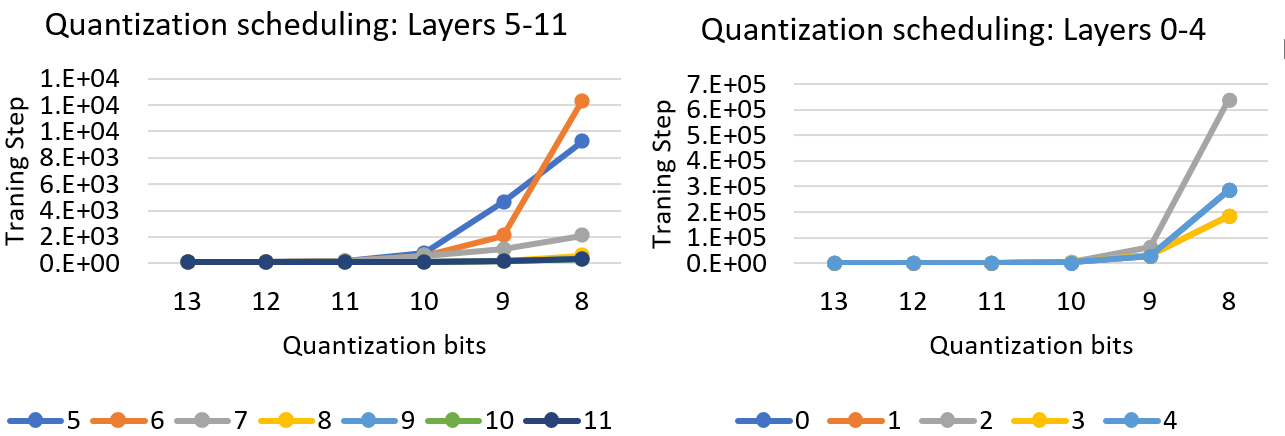
Figure 1. Quantization scheduling of one of the GLUE tasks (QNLI), using the eigenvalue of different layers. Different colors show the layers from 0 to 11 for Bert-Base.

Figure 1 shows the result of combining eigenvalue with MoQ for a 12-layer Bert Base model. As we see, the first few layers (0-4) tend to be more sensitive to reduced precision than the last layers, as their quantization period is an order of magnitude larger than the rest. Another observation from this figure is that the neighbor layers reduce the precision in the same way. For instance, layers 9, 10, and 11 on the left chart, and layers 0 and 4 and 1 and 3 on the right chart of Figure 1 get similar schedule. This is due to having similar eigenvalues for these layers throughout the training.

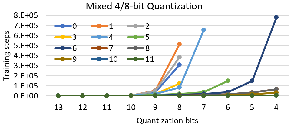Figure 2: Mixed-precision quantization for the QNLI using target quantization period as 4 bits.

Figure 2 shows another mixed-precision quantization that sets target bits as 4, however the quantization period keeps updated through the eigenvalues of each layer. As we see, the end quantization bits are different for all layers. The first layers still get to 8-bit quantization as the training samples is not enough to decrease the quantization bits. On the other hand, the last layers keep reducing the precision. We finally reduce the average precision to 6 bits for the entire network while maintaining the accuracy of the model (0.3% drop in accuracy).

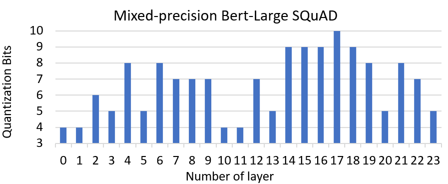Figure 3: Mixed-precision quantization with MoQ for Bert SQuAD plus.

As another example, we use eigenvalue-based MoQ to quantize Bert-Large for SQuAD finetuning. Figure 3 shows the number of bits we get to at the end of finetuning on each layer. Here, we see slightly different precision spectrum compared to BertBase on GLUE tasks. As the figure shows, we can reduce the precision on the first few layers more aggressively than the middle ones. Also, the last few layers can tolerate very low precision similar to the beginning layers. This way of quantization finally results in 90.56 F1 Score which is pretty similar to the baseline.

Quantized Inference Kernels

By using other quantization methodologies, after the model is quantized, it can only have performance benefit if there is hardware support for integer-based operations. For this reason, the inputs and output of all GeMM operations need to be quantized. However, since the range of input may vary request by request, finding a range of data for each input at inference time is challenging. On the other hand, using a static range for all inputs can impact the inference accuracy.

To alleviate this problem, we introduce inference custom kernels that neither require the hardware support nor the input quantization. These kernels read quantized parameters and dequantize them on-the-fly and use the floating-point units of GPU cores for the GeMM operations. The main benefit of using these kernels is that they reduce the memory footprint required to load a model so that we can run inference on fewer number of GPUs, while improving the performance by saving the memory bandwidth required to run the inference on GPU.

Regarding the quantization implementation, we use different algorithms to quantize a value based on the range of data and the rounding policy. We support both symmetric and asymmetric quantization as the two mostly used schemes. We applied both techniques for QAT and see very similar results, however since symmetric approach is simpler to implement, we implement our inference kernels based on that. Regarding the rounding, we support stochastic rounding as another option besides the normal rounding. We have seen that for reducing the precision to as low as 4-bit or lower, stochastic rounding is more helpful as it has an unbiased random behavior during training.

Ease of use

For enabling quantization through Deepspeed, we only need to pass the scheduling through a JSON configuration file. To add the impact of quantization, we quantize and dequantize the parameters just before they are updated in the optimizer. Thus, we do not incur any change on the modeling side to quantize a model. Instead, we simulate the quantization impact by lowering the precision of data saved in FP16 format. By using this kind of implementation, we have the full flexibility of changing the precision using the training characteristics such as number of steps, and eigenvalue of the parameters and the original FP16 data format. As shown in this blog post, we can improve the quality of a quantized model by adaptively changing the scheduling of the quantization throughout training. For more information on how to use MoQ scheme, please look at our quantization tutorial.

Improving quantization accuracy.

To show how our quantization scheme preserves accuracy, we have experimented MoQ on several tasks and networks: GLUE tasks on Bert-Base and SQuAD on Bert-Large. Table 1 shows the accuracy results for the baseline without quantization (w/o Quant), basic quantization without using any scheduling during training (Basic Quant), and our MoQ scheme. Without using any scheduling, the accuracy for 8-bit quantization is often inferior to the baseline, and in this workload, it suffers from a drop of 1.02 point in accuracy (ACC). In contrast, MoQ powers 8-bit quantization to obtain comparable accuracy as the FP16 baseline, even with a slightly higher ACC, demonstrating the effectiveness of our quantization approach.

Task	STSB	MRPC	COLA	WNLI	SST2	RTE	QNLI	QQP	MNLI	SQuAD	ACC+
w/o QAT(FP16)	88.71	88.12	56.78	56.34	91.74	65.3	90.96	90.67	84.04	90.56	0
Basic QAT	88.9	88.35	52.78	55.3	91.5	64.2	90.92	90.59	84.01	90.39	-0.87
MoQ	88.93	89	59.33	56.34	92.09	67.15	90.63	90.94	84.55	90.71	0.75