DeepSpeed Model Compression Library
What is DeepSpeed Compression: DeepSpeed Compression is a library purposely built to make it easy to compress models for researchers and practitioners while delivering faster speed, smaller model size, and significantly reduced compression cost.
Why use DeepSpeed Compression: DeepSpeed Compression offers novel state-of-the-art compression techniques to achieve faster model compression with better model quality and lower compression cost. DeepSpeed Compression also takes an end-to-end approach to improve the computation efficiency of compressed models via a highly optimized inference engine. Furthermore, our library has multiple built-in state-of-the-art compression methods. It supports the synergistic composition of these methods and the system optimizations, offering the best of both worlds while allowing a seamless and easy-to-use pipeline for efficient DL model inference. We highly recommend you also to read our blog to learn more about (at a high level) why we build DeepSpeed Compression and what benefits it provides to users.
How to use DeepSpeed Compression: The first section General Tutorial will describe the compression methods supported by the library. The following sections will describe our research work on how to compose different compression methods to perform zero-cost quantization (ZeroQuant) and extreme compression (XTC). Unless otherwise stated, experiment results listed below are based on NVIDIA A100 GPU, and we observe slightly different result numbers when using different GPU hardwares.
1. General Tutorial
To use DeepSpeed Compression library, you need to install DeepSpeed >= 0.7.0 following the installation guide. Currently the DeepSpeed Compression includes seven compression methods: layer reduction via knowledge distillation, weight quantization, activation quantization, sparse pruning, row pruning, head pruning, and channel pruning. In the following subsections, we will describe what these methods are, when to use them, and how to use them via our library.
1.1 Layer Reduction
What is layer reduction
Neural networks are constructed from input layer, output layer and hidden layer. For example, the BERT-base language model consists of embedding layer (input layer), classification layer (output layer) and 12 hidden layers. Layer reduction means reducing the number of hidden layers while keeping the width of the network intact (i.e., it does not reduce the dimension of the hidden layer). This method can linearly reduce the inference latency of hidden layers regardless of the hardware and/or scenarios.
When to use layer reduction
If the model is very deep, you may consider using this method. It works much better when applying knowledge distillation. Layer reduction can be applied in both the pre-training and fine-tuning stages. The former generates a distilled task-agnostic model, while the latter generates a task-specific distilled model. In our XTC work (paper, tutorial), we also discuss when to apply layer reduction.
How to use layer reduction
Layer reduction can be enabled and configured using the DeepSpeed config JSON file (configuration details). Users have the freedom to select any depth by keep_number_layer and any subset of the network layers by teacher_layer. In addition, users also can choose whether to reinitialize the input/output layers from the given model (teacher model) by other_module_name.
To apply layer reduction for task-specific compression, we provide an example on how to do so for BERT fine-tuning. Layer reduction is about resetting the depth of network architecture and reinitialization of weight parameters, which happens before the training process. The example includes the following changes to the client code (compression/bert/run_glue_no_trainer.py in DeepSpeedExamples):
(1) When initial the model, the number of layers in the model config should be the same as keep_number_layer in DeepSpeed config JSON file. For Hugging Face BERT example, set config.num_hidden_layers = ds_config["compression_training"]["layer_reduction"]["keep_number_layer"].
(2) Then we need to re-initialize the model based on the DeepSpeed JSON configurations using the function init_compression imported from deepspeed.compression.compress.
(3) During training, if KD is not used, nothing needs to be done. Otherwise, one needs to consider applying KD with the teacher_layer JSON configuration when calculating the difference between teacher’s and student’s output.
One can run our layer reduction example in DeepSpeedExamples by:
DeepSpeedExamples/compression/bert$ pip install -r requirements.txt
DeepSpeedExamples/compression/bert$ bash bash_script/layer_reduction.sh
And the final result is:
Epoch: 18 | Time: 12m 38s
Clean the best model, and the accuracy of the clean model is acc/mm-acc:0.8340295466123281/0.8339096826688365
To apply layer reduction for task-agnostic compression, we provide an example on how to do so in the GPT pre-training stage.
Step 1: Obtain the latest version of the Megatron-DeepSpeed.
Step 2: Enter Megatron-DeepSpeed/examples_deepspeed/compression directory.
Step 3: Run the example bash script such as ds_pretrain_gpt_125M_dense_cl_kd.sh. The args related to the pre-training distillation are:
(1)--kd, this enables knowledge distillation.
(2)--kd-beta-ce, this specifies the knowledge distillation coefficient. You can often leave it set to the default value 1, but sometimes tuning this hyperparameter leads to better distillation results.
(3)--num-layers-teacher, —hidden-size-teacher, num-attention-heads-teacher, these parameters specify the network configuration of the teacher model. Please make sure they match the teacher model dimensions in the checkpoint.
(4)--load-teacher, this is where one specifies the teacher model checkpoint.
(5)--load, this is where the initial checkpoint for the student model that is going to be loaded. By default, it will load the bottom layers of the teacher models for initialization, but you can pass your own checkpoints for initialization.
Apart from the above configs, you may also need to modify the data path in the data_options so that the trainer knows the data location. To make things slightly easier, we provide several example scripts for running distillation for different model sizes, including 350M (ds_pretrain_gpt_350M_dense_kd.sh) and 1.3B models (ds_pretrain_gpt_1.3B_dense_cl_kd.sh). We also empirically found that a staged KD often led to a better pre-trained distilled model on downstream tasks. Therefore, we suggest an easy approach to early-stop KD by not setting --kd in the script provided (e.g., disabling KD in the remaining 40% of training).
Step 4: After distilling the model, one can also choose to further quantize the distilled model by running the script 125M-L10-Int8-test-64gpu-distilled-group48.sh, which quantizes both the weights and activations of a distilled model with INT8 quantizer (the weight and activation quantization are introduced in the following sections). note that you need to set the -reset-iteration flag when performing the quantization. We provide the zero-shot perplexity result from WikiText-2 and LAMBADA in the following table.
| GPT (125M) | #Layers | wikitex2 perplexity | LAMBADA |
|---|---|---|---|
| Uncompressed | 12 | 29.6 | 39.5 |
| Quantization only | 12 | 29.8 | 39.7 |
| Distillation only | 10 | 31.9 | 39.2 |
| Distillation + quantization | 10 | 32.28 | 38.7 |
1.2 Weight Quantization
What is weight quantization
Weight quantization maps the full precision weight (FP32/FP16) to the low bit ones, like INT8 and INT4. Quoted from this Coursera lecture: “Quantization involves transforming a model into an equivalent representation that uses parameters and computations at a lower precision. This improves the model’s execution performance and efficiency, but it can often result in lower model accuracy”.
When to use weight quantization
From one-side, again quoted from this Coursera lecture: “Mobile and embedded devices have limited computational resources, so it’s important to keep your application resource efficient. Depending on the task, you will need to make a trade-off between model accuracy and model complexity. If your task requires high accuracy, then you may need a large and complex model. For tasks that require less precision, it’s better to use a smaller, less complex model.”. On the other hand, recent server accelerators, like GPU, support low-precision arithmetic. Therefore, combining weight quantization with activation quantization (introduced in later section) can offer better efficiency as well.
How to use weight quantization
Weight quantization can be enabled and configured using the DeepSpeed config JSON file (configuration details). The key configurations we would like to point out are:
(1)quantize_groups, a group-wise weight matrix quantization: a weight matrix W is partitioned into multiple groups, and each group is quantized separately. See more details in this paper.
(2)quantize_weight_in_forward must be set to true for FP32 optimizer training and false for FP16.
(3)wq1/wq2, users can expand more groups such as wq3, wq4, etc.
(4)start_bit and target_bit, to simplify the first experiment we suggest to set them the same such that we apply quantization to the target bit once the iteration reaches schedule_offset.
There are two changes to the client code (compression/bert/run_glue_no_trainer.py in DeepSpeedExamples):
(1) After initialization of the model, apply init_compression function to the model with DeepSpeed JSON configurations.
(2) After training, apply redundancy_clean function to save the quantized weight.
One can run our weight quantization example in DeepSpeedExamples by:
DeepSpeedExamples/compression/bert$ pip install -r requirements.txt
DeepSpeedExamples/compression/bert$ bash bash_script/quant_weight.sh
And the final result is:
Epoch: 09 | Time: 27m 10s
Clean the best model, and the accuracy of the clean model is acc/mm-acc:0.8414671421293938/0.8422497965825875
1.3 Activation Quantization
What is activation quantization
Activation means the input to each layer. Activation quantization maps the input from full/half precision to low precision. See more in this blog.
When to use activation quantization
It can improve computation efficiency similar to weight quantization.
How to use activation quantization
Activation quantization can be enabled and configured using the DeepSpeed config JSON file (configuration details). Some of the components are same as weight quantization, such as schedule_offset and quantization_type. The key configurations we would like to point out are:
(1)range_calibration, user has option to set dynamic or static. When using “dynamic”, the activation quantization groups will be automatically set to be token-wise (for Transformer-based models) and image-wise (for CNN-based models). See more in our ZeroQuant paper and the code (deepspeed/compression/basic_layer.py in DeepSpeed).
(2)aq1/aq2, users can expand more groups such as aq3, aq4, etc.
The client code change is the same as weight quantization.
One can run our activation quantization example in DeepSpeedExamples by:
DeepSpeedExamples/compression/bert$ pip install -r requirements.txt
DeepSpeedExamples/compression/bert$ bash bash_script/quant_activation.sh
And the final result is:
Epoch: 02 | Time: 28m 50s
Clean the best model, and the accuracy of the clean model is acc/mm-acc:0.8375955170657158/0.8422497965825875
1.4 Pruning
What is pruning
Pruning aims to reduce the number of parameters and operations involved in generating a prediction by removing network connections. With pruning, you can lower the overall parameter count in the network (see more in this Coursera lecture). We can divide the pruning strategy into two types: structured and unstructured pruning (see more in this paper).
| Method | Type |
|---|---|
| Sparse pruning | Unstructured and Structured |
| Row pruning | Structured |
| Head pruning | Structured |
| Channel pruning | Structured |
1.4.1 Sparse Pruning
What is sparse pruning
Sparse pruning means we set some of the elements in each weight matrix with zero values. Relying on the pruning method user chosen, the zero values may have structured pattern or unstructured pattern. One way to perform pruning is based on the absolute value of the weight parameters, see for instance this paper. Another way to perform pruning is based on the weights’ effect to the loss function when they are masked, see for instance this paper.
When to use sparse pruning
If your model is significantly over-parameterized, you may consider using sparse pruning. However, to see the real benefit of hardware computation efficiency, the density ratio (percentage of weights to keep after pruning) must be considerably low.
How to use sparse pruning
Sparse pruning can be enabled and configured using the DeepSpeed config JSON file (configuration details). The key configurations we would like to point out are:
(1)schedule_offset, we empirically find that when using method: topk, it’s better to set the schedule_offset to a large value such as 10% of the total training steps.
(2)method, we support L1 norm, topk and snip_momentum methods. Users are welcome to contribute more methods.
(3)sp1, users can expand more groups such as sp2, sp3, etc. Note this is not needed for snip_momentum method.
(4)dense_ratio, for unstructured sparse pruning, the dense ratio could be less than 0.1 for BRET-base model while still yielding a good accuracy. For ResNet-50, the dense ratio could be as low as 0.3 while still having good accuracy on ImageNet. for structured sparse pruning like snip_momentum, the dense ratio should be specified in shared_parameters and is used to calculate the global sparsity ratio.
(5)frequency, block_pattern and schedule_offset_end, they are used to specify the pruning frequency on steps, the block-wise pruning pattern (NxM and N in M), and the end steps for pruning. For snip_momentum method, these configurations are mandatory.
The client code change is the same as weight quantization.
One can run our sparse pruning example in DeepSpeedExamples by:
DeepSpeedExamples/compression/bert$ pip install -r requirements.txt
DeepSpeedExamples/compression/bert$ bash bash_script/pruning_sparse.sh
And the final result is:
Epoch: 02 | Time: 26m 14s
Clean the best model, and the accuracy of the clean model is acc/mm-acc:0.8416709118695873/0.8447925142392189
1.4.2 Row Pruning
What is row pruning
Row pruning sets all the elements in certain rows of the weight matrix with zero values. If a row is pruned, all elements in that row are set to zero.
When to use row pruning
Row pruning can be beneficial to hardware speedup, much better than sparse pruning (but may result in larger accuracy loss compared to sparse pruning). It is a feature designed for two back-to-back linear layers (e.g., Feed Forward Network in Transformers). As such, we suggested using row pruning for the first linear layer (i.e., the intermediate.dense layer for BERT). Reducing the row dimension of this matrix can help to reduce the column of the follow-up matrix (i.e., layer.\\w+.output.dense layer for BERT). Row pruning would also work for other kinds of linear layers.
How to use row pruning
Row pruning can be enabled and configured using the DeepSpeed config JSON file (configuration details). The key configurations we would like to point out are:
(1)method, only topk method is supported currently. Users are welcome to contribute more methods.
(2)rp1, users can expand more groups such as rp2, rp3, etc.
(3)related_modules, as mentioned in “when to use row pruning”, if we do row pruning, the follow-up matrix will be affected. Thus, one needs to know the connection between the modules.
The client code change is the same as weight quantization.
One can run our row pruning example in DeepSpeedExamples by:
DeepSpeedExamples/compression/bert$ pip install -r requirements.txt
DeepSpeedExamples/compression/bert$ bash bash_script/pruning_row.sh
And the final result is:
Epoch: 02 | Time: 27m 43s
Clean the best model, and the accuracy of the clean model is acc/mm-acc:0.8440142638818136/0.8425549227013832
1.4.3 Head Pruning
What is head pruning
Head pruning is designed specifically for networks with multi-head attention, such as transformer-based models (see more in this blog). For example, the BERT-base (BERT-large) model has 12 heads (24 heads).
When to use head pruning
Head pruning is beneficial to hardware speedup. Moreover, as stated in this blog: “Surprising observations are made in the paper, that even after training models normally (with all heads), many heads can be removed at a test time and it will not significantly affect the BLEU score, in fact, some cases removing few heads led to improving BLEU scores.”.
NOTE: Head pruning is a feature designed for the attention layers (e.g., Multi Head Attention in Transformers). For now, it can only be applied to output matrix of the Transformer (i.e., attention.output.dense in BERT). Pruning the output matrix can lead to the pruning of Query/Key/Value matrix as well.
How to use head pruning
Head pruning can be enabled and configured using the DeepSpeed config JSON file (configuration details). The key configurations we would like to point out are:
(1)num_heads: users need to provide the correct number of heads for their models.
(2)modules: the module attention.output.dense is made specific for Hugging Face BERT model. Currently, we only support this case when Query/Key/Values are separated matrices and followed by attention.output.dense. We are happy to assist and welcome contributions on variants of attention models.
(3)related_modules: as mentioned in “when to use head pruning”, pruning the attention output matrix can lead to pruning QKV matrices as well. Thus, the input here is [“self.query”, “self.key”, “self.value”].
The client code change is the same as weight quantization.
One can run our head pruning example in DeepSpeedExamples by:
DeepSpeedExamples/compression/bert$ pip install -r requirements.txt
DeepSpeedExamples/compression/bert$ bash bash_script/pruning_head.sh
And the final result is:
Clean the best model, and the accuracy of the clean model is acc/mm-acc:0.8397350993377484/0.8377746135069162
1.4.4 Channel Pruning
What is channel pruning
Channel pruning is made specifically for convolutional layers and computer vision. According to wikipedia.org, “The color data of an image is stored in three arrays of values, known as channels.”. For example, an image with three channels passing through ResNet-18 produces 64 channels after the first layer.
When to use channel pruning
Channel pruning is a feature designed for two back-to-back CONV2d layers (e.g., residual connection in ResNet). As such, we suggest using channel pruning for the first CONV2d layer. Reducing the number of output channels of this layer can help reduce the number of input channels of the next layer. Channel pruning would also work for other kinds of CONV2d layers.
How to use channel pruning
Channel pruning can be enabled and configured using the DeepSpeed config JSON file (configuration details).
One can run our channel pruning example in DeepSpeedExamples by:
pip install torch torchvision
DeepSpeedExamples/compression/cifar$ bash run_compress.sh
And the final result is:
after_clean
epoch 10 testing_correct: 0.7664
Note that the above result is when not using batch-norm (BN) in the “ResNet” model. If you use BN for the model and apply channel pruning, the validation after cleaning the model will be different from the model before cleaning. We suggest users to further finetune the model after applying redundancy_clean for such cases.
2. Tutorial for ZeroQuant: efficient and affordable post-training quantization
In this section, we introduce how to apply DS-Compression to perform cost-free INT8 quantization and lightweight INT4/INT8 mixed-precision quantization. For more details, please refer to our paper.
What is ZeroQuant
ZeroQuant is an efficient Post Training Quantization method that includes (1) a fine-grained hardware-friendly quantization scheme for both weight and activations, which can significantly reduce the quantization error; (2) a novel affordable layer-by-layer knowledge distillation algorithm (LKD) even without the access to the original training data; (3) a highly-optimized quantization system backend support to remove the quantization/dequantization overhead. By these techniques, ZeroQuant is able to (1) quantize models to INT8 without any cost and (2) quantize models to INT4/INT8 mixed-precision quantization with minimal resource requirements (e.g., 31s for BERT-base quantization).
When to use ZeroQuant
When you want to quantize the transformer-based model to INT8 or INT4/INT8 format, it is always a good idea to try ZeroQuant first, especially when the model is very resource-hungry (GPU and/or time) to do quantization aware training and/or when the original training data is not accessible.
How to use ZeroQuant
One can run our BERT example in DeepSpeedExamples by:
DeepSpeedExamples/compression/bert$ pip install -r requirements.txt
DeepSpeedExamples/compression/bert$ bash bash_script/ZeroQuant/zero_quant.sh
And the final result is:
Clean the best model, and the accuracy of the clean model is acc/mm-acc:0.8427916454406521/0.8453010577705452
One can run our GPT example by:
DeepSpeedExamples/compression/gpt2$ pip install -r requirements.txt
DeepSpeedExamples/compression/gpt2$ bash bash_script/run_zero_quant.sh
And the final result is:
Before converting the module COVN1D to linear and init_compression: 19.371443732303174
Before cleaning, Epoch at 0 with Perplexity: 19.47031304212775
After cleaning with Perplexity: 19.47031304212775
NOTE: right now, we only support zero cost quantization. Stay tuned for the code release on layer-by-layer knowledge distillation proposed in the ZeroQuant paper.
3. Tutorial for XTC: simple yet effective compression pipeline for extreme compression
In this section, we introduce how to apply DeepSpeed Compression library to perform the light-weight layer reduction and ultra-low bit precision (binary/ternary) quantization. In particularly, we will guide you on implementing the XTC methods, namely:
(1) Obtaining a 1-bit or 2-bit BERT-base (12-layer) with 8-bit activation quantization.
(2) Reducing the 12-layer Bert-base to a 5-layer one and then obtaining its 1-bit or 2-bit counterparts.
What is XTC
XTC (short for eXTreme Compression) is our new simple yet efficient method that compresses a model to its limit with lightweight layer reduction and robust binarization. XTC reduces the model size by 32x with almost no loss in the average score on the GLUE tasks via simple yet effective binarization technique. By combining extreme quantization and lightweight layer reduction, we can further improve the binarized model, achieving 50x model size reduction while keeping 97% of the accuracy. For more details, see how we derive our method in our paper where we perform a systematic study on the impacts of various techniques currently used for extreme compression.
When to use XTC
If you want to significantly compress your models while retaining competitive performance, XTC could be a desirable choice. It is a simple and hyper-parameter tuning friendly method.
How to use XTC
Installation: Examples of XTC extreme compression for BERT models are at compression/bert/bash_script/XTC in DeepSpeedExamples. You will need to install the requirements by:
DeepSpeedExamples/compression/bert$ pip install -r requirements.txt
Implementation of XTC methods:
To accommodate users who do not have a fine-tuned model or task-specific model for compression, with the arg --model_name_or_path yoshitomo-matsubara/bert-base-uncased-${TASK_NAME} our python script run_glue_no_trainer.py automatically downloads the models from Hugging Face. Users can also use their own models with better accuracy as the teacher and the student model initialization.
3.1 One-bit or Two-bit BERT-base (12-layer) with 8-bit activation quantization
For the configurations, see compression/bert/config/XTC/ds_config_W1A8_Qgroup1_fp32.json in DeepSpeedExamples. In our paper, we used FP32 ("fp16": {"enabled": false}) to perform training, while directly applying 8-bit quantization ("bits": 8) to the activations and 1-bit quantization ("start_bits": 1, "target_bits": 1) to the attention (query, key, val) and feedforward weight matrices ("modules": ["attention.self", "intermediate", "output.dense"]) at the beginning of the training ("schedule_offset": 0). In addition, we also apply 1-bit quantization to word_embeddings as weight quantization.
One can run this example by:
DeepSpeedExamples/compression/bert$ bash bash_script/XTC/quant_1bit.sh
And the final result is:
Clean the best model, and the accuracy of the clean model is acc/mm-acc:0.8293428425878757/0.8396053702196908
The other important feature we would like to mention is the quantize_groups inside weight_quantization, which is set to be 1 here to match our XTC paper’s FP32 training setup. We find that under FP16 training, smaller number of quantization group (e.g., 1 or 2) could lead to unstable training. Thus, we recommend using larger number of groups (e.g., 64) under FP16. compression/bert/config/ds_config_W1A8_Qgroup64_fp16.json in DeepSpeedExamples is the FP16 example configurations, where "fp16": {"enabled": true} and "weight_quantization": {"shared_parameters": {"quantize_weight_in_forward": false}} are different from FP32 case.
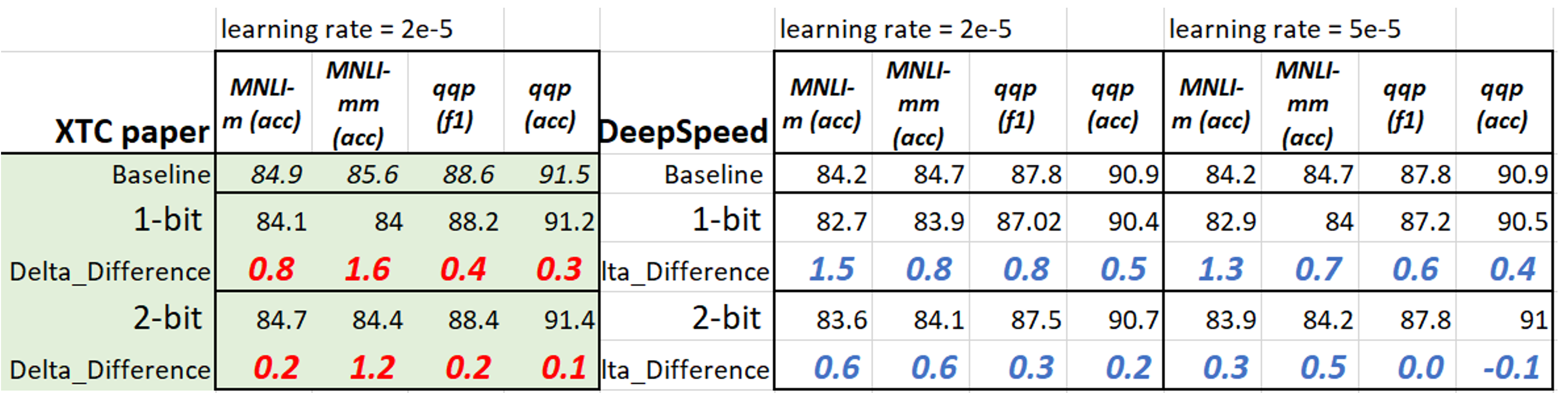
With this config, we quantize the existing fined-tuned models downloaded from Hugging Face. For 2-bit weight quantization, user needs to update the ds_config JSON file. To give a sense of the compression performance of downloaded models compared to our paper, we collect the results (1/2-bit BERT on MNLI and QQP with 18 training epochs) in table below. The difference between this tutorial and paper is because they use different checkpoints. Data augmentation introduces in TinyBERT will help significantly for smaller tasks (such as mrpc, rte, sst-b and cola). See more details in our paper.
3.2 Compressing the 12-layer BERT-base to 1-bit or 2-bit 6/5-layer BERT
This section consists of two parts: (a) we first perform a light-weight layer reduction, and (b) based on the model in (a), we perform 1-bit or 2-bit quantization.
3.2.1 Light-weight Layer Reduction
compression/bert/config/XTC/ds_config_layer_reduction_fp16.json in DeepSpeedExamples is the example configuration for reducing the 12-layer BERT-base to a 6-layer one. The student’s layers are initialized from i-layer of the teacher with i= [1, 3 ,5 ,7 ,9 ,11] (note that the layer starts from 0), which is called Skip-BERT_5 in our XTC paper. In addition, student’s modules including embedding, pooler and classifier are also initialized from teacher. For 5-layer layer reduction, one needs to change the configs in ds_config_layer_reduction_fp16.json to "keep_number_layer": 5, "teacher_layer": [2, 4 ,6, 8, 10](like in compression/bert/config/ds_config_TEMPLATE.json).
One can run this example by:
DeepSpeedExamples/compression/bert$ bash bash_script/XTC/layer_reduction.sh
And the final result is:
Clean the best model, and the accuracy of the clean model is acc/mm-acc:0.8377992868059093/0.8365541090317331
Notably, when using one-stage knowledge distillation (--distill_method one_stage), the difference between the outputs of teacher and student models (att_loss and rep_loss) also need to be consistent with the initialization. See the function _kd_function under forward_loss in compression/bert/util.py.
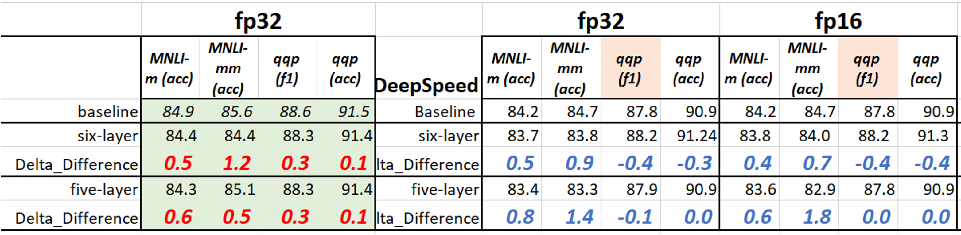
For mnli/qqp, we set --num_train_epochs 36, --learning_rate 5e-5, and with the JSON config above. The results are given below (we also include the fp16 training results). Using fp32 clearly results in more stable performance than fp16, although fp16 can speed up the training time.
3.2.2 One-bit or Two-bit quantization for 6-layer (5-layer) BERT
Given the above layer-reduced models ready, we now continue to compress the model with 1/2-bit quantization. compression/bert/config/XTC/ds_config_layer_reduction_W1Q8_fp32.json in DeepSpeedExamples is the example configuration where we set the layer reduction to be true on top of compression/bert/config/XTC/ds_config_W1A8_Qgroup1_fp32.json. In addition to the configuration, we need to update the path for the student model using --pretrained_dir_student in the script compression/bert/bash_script/XTC/layer_reduction_1bit.sh. User can train with a different teacher model by adding --pretrained_dir_teacher.
One can run this example by:
DeepSpeedExamples/compression/bert$ bash bash_script/XTC/layer_reduction_1bit.sh
And the final result is:
Epoch: 18 | Time: 18m 11s
Clean the best model, and the accuracy of the clean model is acc/mm-acc:0.8140601120733572/0.8199755899104963
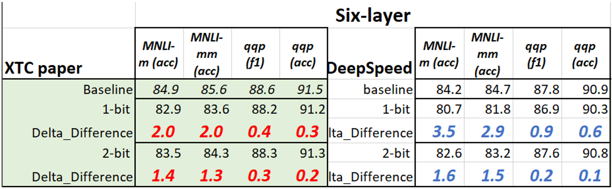
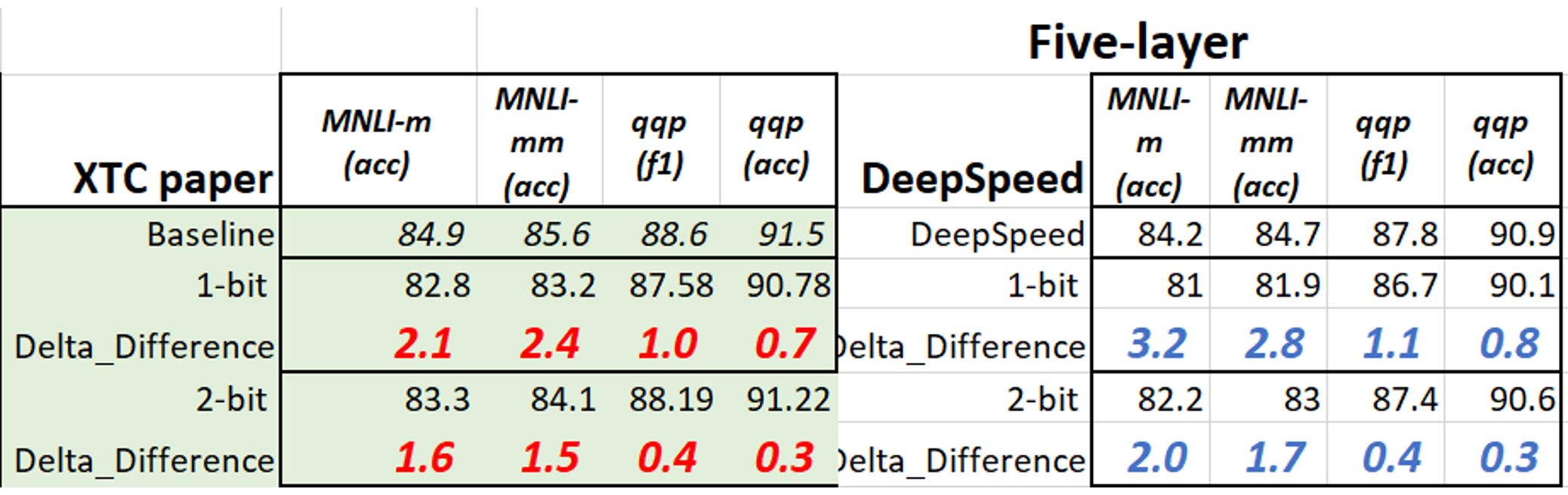
With the command above, one can now obtain the results of 1-bit 6-layer model. Now we list more results for 2-/1-bit 6/5-layer models in the following table. Note that the checkpoints we used for the compression below are from the above table in section 3.2.1.